Using artificial intelligence to search for atmospheric turbulence
Artificial intelligence helps identify gravity waves in the atmosphere. They break similar to waves at the beach and in the process release energy to the atmosphere. In order to quantify this influence, EOC analyses images from high-resolution infrared cameras. AI methodologies help to separate out from the many thousand images for each night those showing turbulence.
Gravity waves arise from oscillations or displacement of the air column, for example whenever air packets are forced to rise over mountain chains. This impulse propagates up to the so-called UMLT (upper mesosphere / lower thermosphere). There atmospheric gravity waves collapse especially frequently and release into the environment the wave energy they transport. The result is that the atmosphere warms up at these locations – and does so to a considerable extent, with consequences for the global weather situation. The behaviour of gravity waves is directly related to the temperature and pressure situation in our troposphere. Deciphering the mechanisms involved can therefore decisively contribute to understanding our climate and climate change.
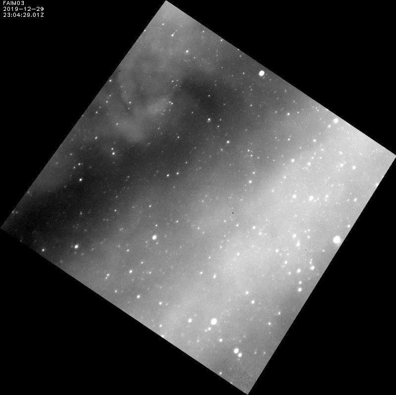
If a wave becomes unstable and breaks, this takes place in connection with turbulence. This phenomenon, experienced during unsteady airplane flights, describes a disorderly, seemingly chaotic airflow. A characteristic of turbulent flow is the formation of vortices, which can also be easily noticed in the smoke emerging from a cigarette. Such swirls also arise in the UMLT in the case of breaking gravity waves and they can be measured with the high-resolution Fast Airglow Imager 3 (FAIM 3) instrument. This is an infrared camera that can be used to monitor from the ground the OH* airglow layer at about 87 km altitude. Air movement in the OH* layer is visible at this altitude. An example of atmospheric turbulence can be seen in the FAIM 3 recordings made in the night from 29 to 30 December 2019 (Video 1): Against the background of the starry night heavens (white dots) there is a swirling structure readily visible in the top corner of the image.

Turbulenzen KI 2021 - Video 1
Your consent to the storage of data ('cookies') is required for the playback of this video on Quickchannel.com. You can view and change your current data storage settings at any time under privacy.
The rotation of turbulent swirls provides information about how much energy is being released to the environment. If the radius and the rotation velocity are read from the images, then it is possible to estimate how much the temperature of the atmosphere rises due to the collapse of a gravity wave. An analysis of several turbulence episodes monitored with FAIM 3 suggests that that can already amount to several Kelvin within just a few minutes. The same heating effect is reached by the chemical processes present in the atmosphere only in the course of an entire day. So that is a clear sign that the dynamic heating caused by breaking gravity waves in the UMLT should be taken seriously and ascertained through continuous measurements.
The ‘big data’ aspect is a major challenge here. Each night images of the OH* layer are recorded automatically every 2.8 seconds by FAIM 3. It is already a laborious and tedious task to search through just a few months of FAIM 3 measurements for indications of turbulence. So how can the examination of a constantly growing mass of data be carried out if even more instruments are put into operation? Here the diffuse structure of the swirls sets limits to classic pattern recognition methodologies.
Therefore, a classification procedure was developed based on neural networks using a well-established artificial intelligence approach. The goal is first of all to reduce the size of the database which has to be examined for cases of turbulence. The images are subdivided into the following three categories for this purpose:
- “Clouds”: images in which the OH* layer is entirely or partly obscured by clouds. These images cannot be used in the analysis.
- “Dynamics”: cloud-free images showing strong movement in the OH* layer.
- “Calm”: cloud-free images of an unperturbed OH* layer.
Images in which turbulence is detected are put into the “Dynamics” category.
A so-called Temporal Convolutional Network (TCN) is used for the automatic classification, whereby the temporal course of the various image parameters is above all also taken into account. This is decisive because it is not always possible to select the category from just one image. The motion category often becomes evident only after looking at a video sequence of several images.
As input, the TCN receives various image parameters expected to be useful in distinguishing the three categories. These include direct information about the image, like the average value of all the pixels, but also parameters that describe the two-dimensional Fourier spectrum or the textures in the image. So that the TCN can learn how to correctly recognize the categories, a so-called training dataset is specified that had been classified – so to speak “by hand” –. by prior manual sorting of the series of images.
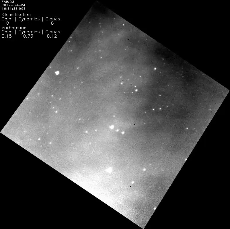
After training, the TCN should be in a position to classify images automatically. An example is shown in Video 2 using brief episodes from the night from 4 to 5 August 2019. The manual sorting is identified in the upper “Classification” table as the number 1. In the lower “Prediction” table the automatic TCN allocation is shown along with its probability. Already at the beginning of the video sequence it becomes clear how well the automatic recognition functions: In the video one first sees considerable movement in the OH* layer – a typical representative of the “Dynamics” category. Starting at 19:44 o’clock a thin veil of clouds passes through the image, which was ignored during manual sorting of the video images. The number 1 in the upper table is still on “Dynamics”. Despite the too coarse manual classification in this case, the TCN nevertheless recognizes the weak cloud signatures and rapidly raises the prediction value for “clouds” to over 0.9. Also, the shifts between the categories “Calm” and “Clouds” after midnight is recognized very well by TCN. By the way, starting at 20:14 o‘clock the formation of a vortex can be seen in the correctly classified “Dynamics” video episode.

Turbulenzen KI 2021- Video 2
Your consent to the storage of data ('cookies') is required for the playback of this video on Quickchannel.com. You can view and change your current data storage settings at any time under privacy.
Thanks to automatic TCN classification it is now possible already in advance to reduce by about 70% the enormous amount of data that has to be examined for turbulence. As a next step, another neural network is to be optimized to automatically identify turbulent vortices in the remaining 30% of the data.
