Rigid helicopter rotor blades – Is this really enough?
July 14, 2022
Rigid helicopter rotor blades – Is this really enough?
Figure 1: Experiment and simulation of the dynamic stall
Left: Rotor test facility Gottingen with four-bladed rotor, right: Aeroelastic numerical simulation of the rotor: Deformed rotor blades surrounded by vortex system
Specially shaped helicopter rotor blades with a kink at the outer part make it possible to reduce the radiating annoying rotor noise [1]. Against this background, the aeroelastic behaviour together with the aerodynamic phenomenon of dynamic stall is of great importance.
Rotor blades with a kink and the dynamic stall
Dynamic stall is generally an aerodynamic stall phenomenon that occurs on wings or aerofoils that experience a rapid change in angle of attack. For helicopters, this condition is given during fast forward flight at the retreating rotor blade which is moving against the direction of flight at that moment. A vortex rolls up on the upper side of the rotor blade which temporarily increases the lift. Afterwards, it moves over the rotor blade before finally being shed. This leads to a sudden and massive breakdown in lift. From an engineering perspective, the rotor blades are therefore exposed to extreme torsional loads and vibrations which additionally stress adjacent components, such as the pitch link rods controlling the pitch angles of the rotor blades.
The dynamic stall in the experiment
In the Rotor Test Facility Göttingen (RTG) [2, 3] operated by the DLR Institute of Aerodynamics and Flow Technology dynamic stall is brought about in a specific experiment on the ground, see Fig. 1 left. For this purpose, the kinked model rotor blade [4] runs through a well-defined pitching motion on the rotor test bench including one up- and downstroke in each rotor revolution. The experiments are accompanied by numerical simulations which additionally include the elasticity of the rotor blades besides purely rigid modelled ones, see Fig. 1 right.
The aeroelastic simulation method
In aeroelastic simulations, different numerical solution techniques are usually applied in both subfields of structural and fluid mechanics. On the one hand, a multibody system (MBS) represents the structural mechanics of the model rotor by means of individual interconnected rigid and elastic bodies [5], on the other hand, the solution of aerodynamic flow is calculated using computational fluid dynamics (CFD). A special feature in the simulation of helicopter rotors are moving CFD grids allowing to reproduce the complex motions of the rotor blades. The so-called Chimera technique includes in this case four rotor blade grids moving in a large background grid. At their outer boundaries, the rotor blade grids permanently exchange solution data with the background grid so that, as an example, generated vortices can be shed from the rotor blades into the flow field, see Fig. 1 right. Finally, a coupling algorithm connects both subfields by exchanging aerodynamic forces and structural deformations at the rotor blades [6, 7].
Rigidly and elastically modelled blades differ from each other
Figure 2: Hysteresis loops for the blade normal force
Analogous to aircraft wings, which do not perform any pitching motion during cruise flight, the aerodynamic loads as well as structural deformations are typically plotted against the pitch angle Θ of the rotor blade. Therefore, Figure 2 shows the blade normal force (aerodynamic load) in case of a rigid and elastic blade modelling. The difference in the curve progression between the up- and downstroke motion is striking and a defining feature of the hysteresis that sets in with dynamic stall. The red (= rigid) and green (= elastic) curves clearly show that the hysteresis behaviour depends on the inclusion of elasticity in the modelling of the blades.
Frequency analysis allows deeper insight into what is happening
All aerodynamic and structural blade loads change during one rotor revolution however they return exactly after each one. This is exploited by describing them mathematically as a sum of several sine and cosine functions with frequencies of the rotor speed as well as its integer multiples, i.e. 2, 3, 4, ... times. These are the so-called rotor harmonics which are numbered according to the multiple, see Fig. 3. They provide more detailed information and contribute to a deeper understanding, as all events contained in the stall phenomenon can now be analysed individually, separated according to their frequency.
Although the stall phenomenon occurs solely once per rotor revolution corresponding to the first rotor harmonic, the frequency analysis shows that the aerodynamic loads also include higher rotor harmonics. For the normal blade force, the first five are of essential importance, see Fig. 3 left. The afore-mentioned differences in aerodynamic loads between rigid and elastic blade modelling can now be narrowed down primarily to the contributions of the first and second rotor harmonics. Interestingly, the oscillatory motion of the blade tip also consists mainly of both rotor harmonics mentioned, see Fig. 3 right. Their dominant participation in this can also be observed in the experiment.
Figure 3: Rotor harmonics in frequency spectrum
Left: Blade normal force, right: Blade tip deformation
To understand the problem in its entirety one should get to the bottom of the following question: Why does the rotor blade have a vibration component with double the rotational frequency?
Campbell diagram
In a rotating rotor, the natural frequencies often depend on its speed as they are influenced by gyroscopic effects and centrifugal forces. Accordingly, a Campbell diagram illustrates the mentioned relation by plotting the natural frequencies against rotor speed. Together with the rotor harmonics, which appear as straight lines, possible resonances can be found. In these cases, the frequencies of excitation and natural oscillation are the same which results in an intersection point between a curve of a rotor harmonic and a natural frequency. Under further conditions, the actual occurrence of resonance shows high oscillation deflections in the rotor blades which, moreover, can already be brought about by small excitation forces.
The Campbell diagram in Fig. 4 reveals an intersection point near the rotor speed selected in the experiment. Here, the frequency curve of the first bending natural oscillation intersects with the straight line of the second rotor harmonic, so that at this operating point the rotor blade is effortlessly made to oscillate at double the rotational frequency. The vibrational motion of the rotor blade is accompanied by changes in the aerodynamic inflow conditions which essentially contribute to its normal force. This effect can be described in more detail using the frequency analysis again:
Due to the vibrational motion with a predominant first and second rotor harmonic, mainly the contributions of the first and second rotor harmonic change in the normal force as depicted in Fig. 3, too.
Conclusion on aeroelastic simulation
With the help of the aeroelastic simulation, additional effects can be depicted during the dynamic stall event that are attributable to the vibration behaviour of elastic rotor blades. Their influence on the aerodynamic loads can thus be determined in order to make more accurate predictions in the development of future rotor blades. It is therefore necessary to model rotor blades elastically – rigid helicopter blades are not enough!